← Back to articles
AI-Native Equity Risk Dashboard with Claude Code
Originally published on medium.com
Building an AI-Native Equity Risk Dashboard with Claude Code and RiskModels
Claude Code can build the interface in minutes. The harder question is whether the interface knows anything real about equity risk.
Ask Claude Code to build a stock-risk dashboard and it will usually produce something polished: a ticker input, a rolling-volatility chart, a correlation matrix, perhaps a beta against SPY.
The application may compile. The charts may look professional. But the result is still limited by the information available to the agent.
A coding agent is a builder, not a risk model.
Without a structured source of domain knowledge, it can calculate familiar statistics from price history. It cannot reliably determine how much of a position’s risk comes from the market, its sector, its subsector, or the stock itself — or which liquid ETF hedges each layer.
That is the distinction this project tests.
I connected Claude Code to the RiskModels MCP server, gave it an intentionally incomplete prompt, and asked it to build an interactive dashboard around ERM3, RiskModels’ hierarchical equity-risk model.
Here’s what Claude built in about five minutes
Claude did not invent a risk model. It assembled a front end around one. On the live vintage used for this article (data as of 2026–07–14), the comparison view already shows why that matters:
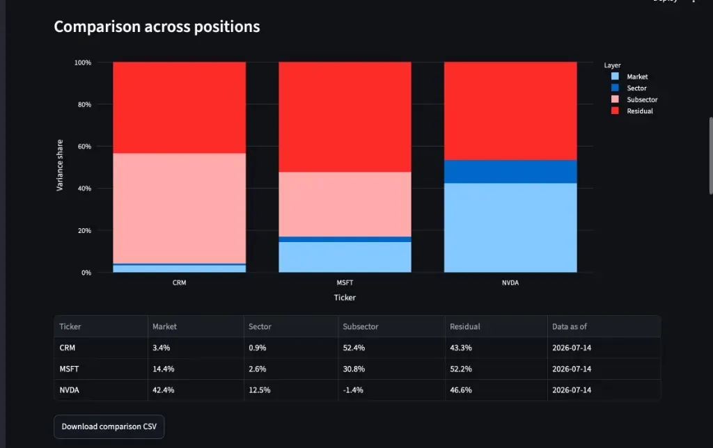
CRM, MSFT, and NVDA on the same model date. Similar total volatility would not reveal that CRM and MSFT are subsector- and residual-heavy while NVDA carries far more market share.
That screen is the payoff. Everything below is how it got there — and why the agent still needed a domain API to get the answers right.
How the pieces connect
The loop is short: a prompt to Claude Code, MCP tools against RiskModels, one ERM3 call, a Streamlit UI.
Prompt → Claude Code → RiskModels MCP → /decompose → Dashboard
RiskModels exposes ERM3 through REST, Python, CLI, and MCP (https://riskmodels.app/api/mcp/sse). Install locally with npx -y riskmodels@latest install. The endpoint for this project is POST /api/decompose: four additive variance layers (market, sector, subsector, residual), each with er, hr, and hedge_etf, plus a signed hedge map. The four ER shares sum to ≈ 1. Residual has no ETF hedge—it is unexplained variance, not alpha.
The prompt — and the mistake that revealed the lesson
I deliberately did not give Claude a detailed UI specification. The point was to see what it could infer once it had access to a real risk schema.
Build a Streamlit dashboard using the RiskModels decomposition API. Let the user compare several tickers, inspect the four ERM3 risk layers for one stock, see the ETF hedge notionals per $1 long, and visualize which risk remains after applying an L1, L2, or L3 hedge. Validate the API response and explain residual risk correctly.
Claude handled the scaffolding well: Streamlit layout, cached calls, validation, comparison views, readable hedge trades.
But the first version made a revealing conceptual mistake: it described residual risk as “uncaptured alpha.”
That phrase sounds plausible. It is also wrong. Residual ER is a variance share with no sign and no claim about future returns.
One corrective prompt fixed the label. The lesson stuck: the agent is excellent at constructing software and weak at inventing financial meaning that was not encoded in the tools or instructions.
What the dashboard answers
1. What is the position actually exposed to?
For CRM on the same vintage:
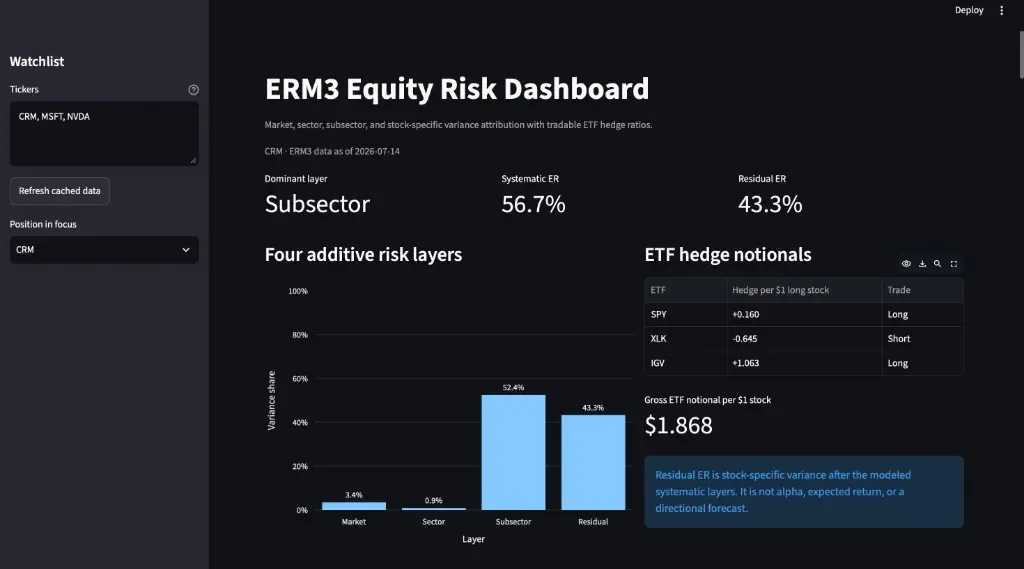
Market 3.4%, sector 0.9%, subsector 52.4%, residual 43.3%. Subsector (IGV) dominates; a single-factor SPY beta would miss that.
A conventional beta compresses the position into one market relationship. ERM3 asks whether variation associates with the broad market, the sector, a narrower subsector, or the stock itself.
2. Which ETFs hedge those layers?
For each $1 long CRM:
SPY   +0.160
XLK   -0.645
IGV   +1.063
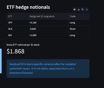
Signed ETF notionals per $1 long stock: positive = long the ETF, negative = short it.
Those signs follow from how ERM3 is estimated. The model fits market, then sector, then subsector as a sequential orthogonal cascade: each layer’s hr measures incremental exposure after broader layers are removed—not a univariate OLS beta on that ETF alone. The /decompose hedge map flips each tradable layer’s hr (negative of hr, duplicates summed), so the numbers above are dollars of ETF per $1 long stock. For CRM that is SPY +0.160, XLK −0.645, IGV +1.063—long SPY and IGV with a short XLK leg. Standalone betas can disagree with those signs because XLK and IGV share market/tech exposure already partialed out upstream. Read the hedge map; do not reconstruct the trade from univariate intuition.
3. What remains after each hedge depth?
- No hedge retains all four layers.
- L1 removes market.
- L2 removes market and sector.
- L3 removes market, sector, and subsector.
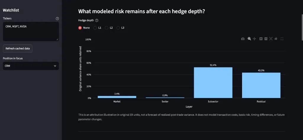
Unhedged baseline (Hedge depth = None): all four CRM layers still present. Selecting L1 / L2 / L3 zeros market, then sector, then subsector — after L3 only residual remains in these ER units, not because residual became 100% of variance, but because the modeled systematic layers were zeroed.
This is an attribution view, not a promise of realized hedge performance.
4. Why does CRM behave differently from MSFT?
Once the panels exist, the interesting question is interpretive — and that is where a coding agent grounded in the model starts to sound like it understands risk rather than merely charting it:
User:
Why is CRM behaving differently from MSFT?
Claude:
CRM's risk is primarily concentrated in the IGV subsector,
whereas MSFT still carries substantially more market exposure.
A market hedge removes relatively little CRM variance.
An IGV hedge removes far more.
That answer is not a vibe from price charts. It is a readout of the same structured layers the dashboard renders.
You don’t have to trust the agent’s charting either
There is a second trust boundary this project surfaced. The screenshots above are the Streamlit UI Claude built — Plotly defaults, layout choices, and all. Even with correct /decompose numbers, an agent-drawn chart is still the agent's interpretation of scale, ordering, and emphasis.
RiskModels closes that gap the same way it closes the data gap: the platform also serves its own canonical panels. The same CRM / MSFT / NVDA vintage is addressable, unmodified, from
GET /api/snapshot/stock/{ticker}/panels/{slug}?format=png
with slugs l3_explained_risk_hbar, hedge_notionals_hbar, hedge_depth_retained, and watchlist_er_stacked (pass tickers=CRM,MSFT,NVDA for the watchlist panel). These are registry artifacts—versioned render code maintained with the model—not notebook plots. An agent can embed those bytes instead of reinventing the charts, which means a production dashboard and the platform's own research artifacts can never quietly disagree.
The code
The core call is intentionally straightforward:
@st.cache_data(ttl=3600)
def get_decomposition(ticker: str) -> dict:
    response = requests.post(
        "https://riskmodels.app/api/decompose",
        headers={"Authorization": f"Bearer {API_KEY}"},
        json={"ticker": ticker},
        timeout=30,
    )
    response.raise_for_status()
    payload = response.json()
    validate_decomposition(payload)
    return payload
Validation checks that all four layers exist, ERs are numeric and sum near 1.0, and the hedge object has the expected shape. AI-generated apps should not silently assume every payload is complete.
Hedge-depth views operate on the additive layers directly — zeroing market, then sector, then subsector — without pretending to recompute a future covariance matrix. The full Streamlit app ships with this article.
Why MCP matters
MCP lets the agent discover tools, inspect schemas, call them while working, and revise the UI around real responses — instead of copying field names from docs.
That is a stronger loop than ordinary REST integration. With a hard-coded HTTP client, the developer still has to know which endpoints exist, what their schemas mean, and how to interpret each field. With MCP, Claude can enumerate available operations, read structured capability descriptions, invoke tools while scaffolding the app, and iterate against typed responses — working inside the platform’s tool surface, not merely pasting a URL into requests.post.
Responsibilities stay separated: Claude Code builds the interface; RiskModels supplies the domain model and current data; the developer verifies interpretation. The result is not autonomous financial expertise. It is a faster way to assemble software around an explicit, inspectable source of expertise.
Where this can go next
The four panels above are the entry point to a deeper surface. The same platform composes them — plus peer risk-DNA comparisons, return-decomposition waterfalls, and fundamentals trajectories — into a full institutional deep-dive page:
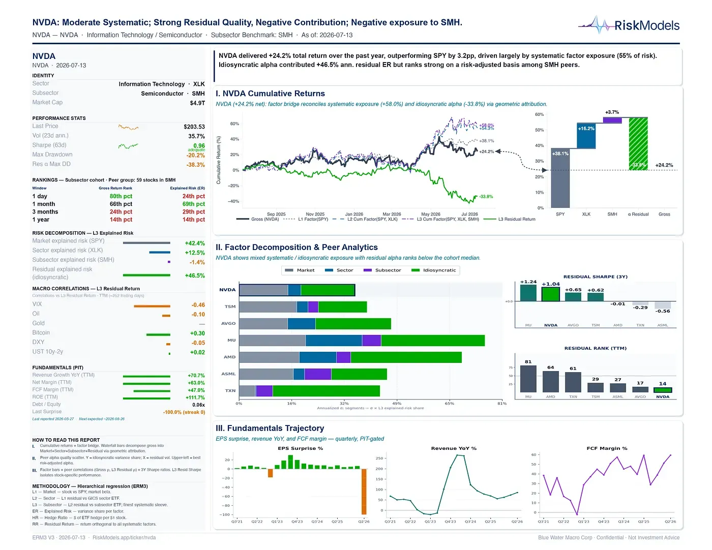
The institutional one-pager for NVDA (live; the vintage shown here is 2026–07–13; dashboard figures above are 2026–07–14). The panels in this article are the addressable pieces of the same kind of analysis.

Richer builds stay on the same boundary: portfolio tables ranked by residual share, holdings-weighted hedge notionals, drift alerts, return decomposition, natural-language explanations grounded in ERM3. The important step is not adding more charts. It is preserving what the agent generates versus what the domain system knows.
Takeaways
Coding agents generate software. They do not generate financial truth.
A polished chart built from an improvised beta is still an improvised beta. Connecting the agent to a documented model changes the quality of the result because it gives the software an explicit structure to represent.
The dashboard was always going to be built quickly. That is what coding agents are good at.
The meaningful difference is that its market, sector, subsector, residual, and hedge fields come from a real equity-risk model rather than from plausible-looking calculations invented inside the application.
As coding agents become ubiquitous, competitive advantage shifts away from writing software and toward owning structured, machine-readable expertise. In quantitative finance, that expertise is the model.
The same agent-plus-MCP pattern extends naturally beyond /decompose—and much of that surface is already live: point-in-time fundamentals with cost-of-capital derived from the same betas (GET /api/fundamentals/{ticker}, with MCP and SDK clients), mutual-fund and 13F-filer snapshots, style-cohort rankings, and the addressable research panels used above. Decomposition is a clean first project; the larger idea is an AI-native quantitative research platform where coding agents are front ends to structured market expertise rather than authors of that expertise.
Get started
Local Claude Code / Cursor installation:
RISKMODELS_API_KEY=your_api_key_here npx -y riskmodels@latest install
Python SDK:
python3 -m pip install "riskmodels-py>=0.3.4"